
Now let’s move on to more advanced datastructures. You are familiar with queues (first in first out, FIFO) and stacks (first in last out, FILO), and they have tons of examples in real life. But what about a priority queue? What are real-life examples of a priority queue (PQ)?
The best example of a priority queue is the emergency room (ER) in a hospital, and I hope you will never need to go there because if you ever go there, you will likely have to wait for a really long time. During this waiting period, you will see many people arriving after you but got treated before you, and thought that’s really unfair! But the reality is, it is not a queue, but a priority queue, so each time a doctor becomes available, she will treat the patient in the waiting room who has the highest priority (i.e., most urgent). Because most of my readers are young students, I assume it is highly unlikely that you are ever very ill and get assigned a high priority, so it is natural that you need to wait for a long time. In fact, you would even hope your priority is low, because you don’t wanna get very sick!
Another interesting fact about the ER is that the priorities can change over time. When you first come in, you’re assigned an initial priority, but as time goes by, if you don’t get treated, it is possible that your situation worsens and your priority goes up (assuming the nurse periodically assesses people in the waiting room). On the other hand, it is also possible that over time, your acute illness becomes alleviated naturally, then your priority goes down (for example, many years ago I went to the ER for some reason that I no longer remember, and had to wait there forever, but after 3 hours, I felt not as bad as when I first came, and just went home).
This “dynamic” priority is a very interesting but rather advanced feature and is used in two famous graph algorithms that require a priority queue with this feature: the Dijkstra algorithm for shortest path and its close relative Prim’s algorithm for minimum spanning tree, which we will see in Chapter 3.
Most priority queue implementations, however, only support static priorities, but that’s enough for all applications in this Chapter.
A priority queue is an abstract data type (like a Java interface that can be implemented with different concrete data structures such as binary heap or sorted array (which, in the Java terminology, implements the priority queue interface). An abstract data type specifies a few functions (with signatures) that a concrete data structure must implement. For example, a priority queue must support the following operations:
Next we will see that different implementations of PQ have very different running times for these operations.
While we all know that binary heap is the default implementation for PQ, it is not the only possible one. In fact, you can also implement a PQ by a sorted array, an unsorted array, an inversely sorted array, etc.
We can see that all these implementations would suffer from an \(O(n)\) operation in either push or pop. If we use these implementations to do sorting with PQ, it would cost \(O(n^2)\) time. But we know sorting can be done in \(O(n\log n)\) time, so can we make push/pop operation \(O(\log n)\) instead? What does \(O(\log n)\) remind you? Binary search, and balanced binary search tree! Yes, we should use balanced tree structures to implement a PQ, because the height is bounded by \(O(\log n)\). Indeed you can use a self-balancing binary search tree, but there is another, much simpler, data structure that is more suitable for PQ: binary heap.
Binary heap belongs to a very specialized subtype of balanced binary trees called complete trees, in which every level, except possibly the last, is completely filled, and all nodes in the last level are as far left as possible.
Why is complete trees even better than general balanced trees? We’ll see below that they are much more convenient to be represented (or “linearized”) as arrays (via level-order traversal), and arrays are much more efficient to manipulate than trees.
How would we organize the ER patients in such a tree? Naturally, the root is the most urgent (highest priority) patient, so that peek is \(O(1)\). By default we talk about min-heaps (but you can also use max-heaps), where the root is the smallest. In terms of priority (urgency) in ER, think about it as a number meaning “distance to death”, so a smaller number indicates higher priority. What about the rest of the heap? Well, each node needs to be smaller than both children (or actually, all descendents, i.e., in each subtree, the root is the smallest). Like other structures such as BSTs, heap can also be defined recursively:
When performing the operations, we need to maintain both the shape property (complete tree) and heap property (each node is smaller than both children).
initial min-heap:
        1
      /   \
     2     4
    / \   /
   8   5 6

push 0 (append at the end):
        1
      /   \
     2     4
    / \   / \
   8   5 6  *0*

violation. swap with 4
        1
      /   \
     2    *0*
    / \   / \
   8   5 6   4

still violation. swap with 1
       *0*
      /   \
     2     1
    / \   / \
8 5 6 4 *4* *4* *4*
/ \ / \ / \
2 3 5 3 3 5But in any case, we should choose the smallest out of the three numbers (root, left node, right node) and swap that number with the root:
    2      3        3
   / \    / \      / \
 *4*  3  5  *4*  *4*  5
and keep going down the tree until no longer violating the heap property. Here is a complete example of pop:
initial min-heap:
        1
      /   \
     2     4
    / \   /
   8   5 6

pop (return 1, replace it with 6):
       *6*
      /   \
     2     4
    / \
   8   5

violation. bubble-down, swap with 2
        2
      /   \
    *6*    4
    / \
   8   5

still violation. bubble-down, swap with 5
        2
      /   \
     5     4
    / \
   8  *6*
Because heaps are complete trees which are in turn balanced trees, the height is \(O(\log n)\), thus both push and pop are \(O(\log n)\) time.
As hinted above, although heaps are trees, they can be more efficiently stored in arrays thanks to the complete tree property, so that the linearized version using level order traversal is a consecutive sequence (this would not be possible if the tree is not a complete tree).

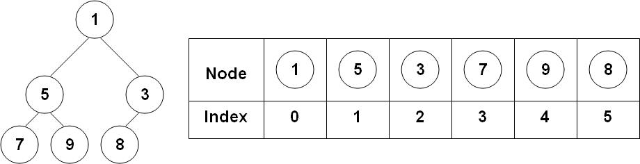
The nice thing about this linearized representation is that we can locate children and parent via indexing. For each element at index \(i\) (in a 0-based index like C/Java/Python):
(i-1)//2 in Python3).This way bubble-up and bubble-down operations can be made extremely fast.
heapq moduleFor example, the builtin heapq module in Python is an
efficient and lightweight array implementation of a min-heap.
>>> import heapq
>>> h = [] # empty queue
>>> heapq.heappush(h, 5)
>>> heapq.heappush(h, 2)
>>> heapq.heappush(h, 4)
>>> heapq.heappush(h, 8)
>>> heapq.heappush(h, 1)
>>> heapq.heappush(h, 6)
>>> h
[1, 2, 4, 8, 5, 6]
>>> h[0] # peek
1
>>> heapq.heappop(h) # returns root
1
>>> h
[2, 5, 4, 8, 6]
This example is identical to the one above.
Another very useful function is heapreplace() which is
conceptually a combination of heappop() and
heappush(), but is more efficient because it just replaces
the root by a new element, followed by a bubble-down:
>>> heapq.heapreplace(h, 9) # pops root, replaces it by 9
2
>>> h
[4, 5, 9, 8, 6]
Yet another useful function is heapify(), which builds a
heap from an existing list (instead of calling heappush()
\(n\) times).
Given an unsorted array, how do you quickly make it into a heap? A
real-life scenario would be that many patients arrive at (an empty) ER
at the same time (for example, from an accident). Obviously you can push
them into the heap one-by-one as we did in the above example of
heapq, but this would cost \(O(n\log n)\). Can you do it slightly
faster? Indeed we can: heapify is \(O(n)\).
heapify as
divide-n-conquer (top-down)Let’s first view heapify as divide-n-conquer. A random
array is still a complete tree in our linearized representation of
heaps, e.g.:
            5
         /     \
        2       6
      /   \    / \
     1     4  3   7
    / \   /
   8   0 9
But it’s clearly not a heap. How should we make it a heap? Just divide-n-conquer, in a post-order traversal:
You can call heapify(heap) as defined
below:
def heapify(heap, i=0):
    if 2*i+1 >= n: # leaf node?
        return
    heapify(heap, 2*i+1) # heapify left tree
    heapify(heap, 2*i+2) # heapify right tree
    bubbledown(heap, i) # adjust root
The runtime recurrence would be:
\[T(n) = 2T(n/2) + O(\log n)\]
because the tree height is \(O(\log n)\). We will see how to solve it to \(O(n)\) below.
heapify as bottom-upSince the above top-down heapify is a post-order
traversal, the real execution is in bottom-up order. Note that leaf
nodes are already heaps, so we just need to adjust the
[1,8,0] tree first by a 1-step bubble-down:
            5
         /     \
        2       6
      /   \    / \
     0     4  3   7
    / \   /
   8  *1 9
Its sibling [4,9] tree doesn’t need adjustment. So we
backtrack at node 2 which needs a 2-step bubble-down:
            5
         /     \
        0       6
      /   \    / \
    *2     4  3   7
    / \   /
   8   1 9

            5
         /     \
        0       6
      /   \    / \
     1     4  3   7
    / \   /
   8  *2 9
Now the left subtree of the root is a heap, so we visit its sibling,
the [6,3,7] subtree, and need a 1-step bubble-down:
            5
         /     \
        0       3
      /   \    / \
     1     4 *6   7
    / \   /
   8   2 9
Now both left and right subtrees are done, and the only remaining step is to bubble-down from the root, which needs 3 steps:
            0
         /     \
       *5       3
      /   \    / \
     1     4  6   7
    / \   /
   8   2 9

            0
         /     \
        1       3
      /   \    / \
    *5     4  6   7
    / \   /
   8   2 9

            0
         /     \
        1       3
      /   \    / \
     2     4  6   7
    / \   /
   8  *5 9
So the final array is [0, 1, 3, 2, 4, 6, 7, 8, 5, 9]
which is identical to the result of heapq.heapify.
>>> h = [5, 2, 6, 1, 4, 3, 7, 8, 0, 9]
>>> heapq.heapify(h)
>>> h
[0, 1, 3, 2, 4, 6, 7, 8, 5, 9]
We can also express this bottom-up process in a (backwards) loop,
from index |h|//2 - 1 (the first node with children) downto
0 (root). This is because the bottom half of the array are
all leaf nodes which do not need adjustment (or base cases of
recursion). To be precise, for node with index \(i\), its left child is at index \(2i+1\), so we need \(2i+1 \leq |h| -1\) for node \(i\) to have children. Therefore
\[ 2i+1 \leq |h| -1 \Rightarrow 2i \leq |h| - 2 \Rightarrow i \leq \frac{|h|}{2} - 1 \]
For the above example with |h|=10 nodes, we have
i <= 10//2 -1 = 4. So the first node to adjust is
h[4]:
     index: 0  1  2  3  4  5  6  7  8  9
       h = [5, 2, 6, 1, 4, 3, 7, 8, 0, 9]
non-leaves <-------------||-------------> leaves
            5
         /     \
        2       6
      /   \    / \
     1    4<- 3   7
    / \   /
   8   0 9
Indeed, this node is the first one that has children in the backward
order. All nodes after it in the linear order are leaf nodes (half of
the array). So we can write a simple loop, which is how
heapify is implemented in practice:
def heapify2(h):
    for i in range(len(h)//2-1, -1, -1): # downto 0
        bubbledown(h, i)
Tree Traversal Orders:
heapify2() above uses
reverse level-order traversal.heapify() above uses post-order traversal.heapify is \(O(n)\) [advanced]High-level intuition why heapify is faster than \(n\) heappushes:
Now let’s analyze heapify more carefully:
In general, \(n/2^{i+1}\) nodes have height \(i\) (\(i=0\ldots h\) with \(h=\log n-1\)). So the total work is:
\[ \begin{align} & n/2 \cdot 0 + n/4 \cdot 1 + n/8 \cdot 2 + \ldots + n/n \cdot (\log n - 1)\\ = & n \cdot (0 + 1/4 + 2/8 + 3/16 + \ldots + h/2^{h+1}) \end{align} \]
Here \(1/4 + 2/8 + 3/16 + \ldots\) is a very interesting series called arithmetico-geometric sequence because the numerator is arithmetic while the denominator is geometric (see also here and here). It still converges:
\[ \begin{align} & 1/4 + 2/8 + 3/16 + 4/32 +\ldots \\[0.1cm] =& 1/4 + 1/8 + 1/16 + 1/32 +\ldots \\ &+\!\! 0 + 1/8 + 2/16 + 3/32 +\ldots \\[0.1cm] =& 1/4 + 1/8 + 1/16 + 1/32 +\ldots \\ &+\!\! 0 + 1/8 + 1/16 + 1/32 +\ldots \\ &+\!\! 0 + \ \ 0 \ + 1/16 + 2/32 + \ldots \\[0.1cm] =& 1/4 + 1/8 + 1/16 + 1/32 +\ldots \\ &+\!\! 0 + 1/8 + 1/16 + 1/32 +\ldots \\ &+\!\! 0 + \ \ 0 \ + 1/16 + 1/32 + \ldots \\ &+\!\! 0 + \ \ 0 \ + \ \ 0\ \ \ + 1/32 + \ldots \\ &+\ldots \\[0.1cm] =& 1/2 + 1/4 + 1/8 + 1/16 + \ldots\\ =&1 \end{align} \]
An alternative method for solving this series (let’s call it
x) is to observe (from the second line above):
\[ x = (1/4+1/8+1/16+1/32 + \ldots) + x/2\]
and therefore \(x = 1/2 + x/2\) and \(x=1\).
So heapify is \(O(n)\) time.
Note that these two derivations are much simpler than the ones in most textbooks (such as CLRS) which require calculus.
heapify and \(n\) heappush’s:To see if this analysis makes a difference in practice, I wrote a little program to compare them on the worst-case input (inversely sorted array, so that you need to bubble-down all the way to the leaf node or bubble-up all the way to the root):
import time, heapq

for i in range(5):
    n = 1000000 * 2**i
    a = list(range(n, 0, -1)) # worst-case input
    h = a.copy()
    t = time.time()
    heapq.heapify(h)
    t1 = time.time()
    h = []
    for x in a: heapq.heappush(h, x)
    t2 = time.time()
    print("n=%9d heapify: %.4f  n heappushes: %.4f ratio: %.2f" % (n, t1-t, t2-t1, (t2-t1)/(t1-t)))
and the difference is huge:
$ python3 test_heapify.py
n=  1000000 heapify: 0.022  n heappushes: 0.294 ratio: 13.6
n=  2000000 heapify: 0.043  n heappushes: 0.617 ratio: 14.4
n=  4000000 heapify: 0.088  n heappushes: 1.270 ratio: 14.5
n=  8000000 heapify: 0.171  n heappushes: 2.650 ratio: 15.5
n= 16000000 heapify: 0.342  n heappushes: 5.476 ratio: 16.0
You can see that heapify is much faster, and as \(n\) grows, its advantage is bigger (\(O(n)\) vs. \(O(n\log n)\)).
Dynamically changing priorities is a more advanced topic used in graph algorithms such as Dijkstra’s (shortest-path) and Prim’s (minimum spanning tree), so we’ll discuss it in Chap. 3. For the classical applications of priority queues discussed in the next section, static priority is good enough.
Binary heap and heap sort were invented by British computer scientist JWJ Williams in 1963. Further improvements of heap include the Fibonacci heap, which improves push to \(O(1)\), but it’s too complicated for practical use.